
Types of Waves
There are many types of waves in this world. Water waves and sound waves are well known to the average person. The waves that are better known to scientists include seismic waves, structural waves, light and other forms of electromagnetic radiation, quantum mechanic pilot waves, magnetic spin waves, and waves in plasmas. In this posting we hope to give an overview of some of the ways waves are classified. We start with classifying by the number of dimensions, i.e. 1D, 2D, or 3D waves.
A wave on a string is an example of a one dimensional wave as shown to the left. Mouse over the image to see the action. These waves travel along a line, i.e. along a one dimensional space. These waves are only a function of one space variable, such as x, in addition to time, t. They satisfy the one dimensional wave equation:
one dimensional wave equation
where c is the speed of the wave propagation. These have solutions of the form y(x, t) = f(x ±ct), i.e. d’Ambert’s solutions.
These solutions include pulses, gaussians, and any shape function that travels to the left or right at the speed c. We are often more interested in sinusoidal and complex exponential solutions, i.e. the sine, cosine or exp forms given by
y(x, t) = Asin(κx − ωt) , y(x, t) = Acos(κx − ωt), or y(x, t) = Aei(κx − ωt) .
Remember that the wave number is defined as
κ = ω/c .
(A discussion of variables such as ω is found at this link. A discussion of simple waves and wave numbers κis found at this other link.)
Waves in two dimensions
Waves can also travel on a surface that is a two dimensional space, such as the surface of water or in a layer of clouds as shown below. These are examples of two dimensional (2D) waves. While one dimensional waves are easiest to understand and analyze, two dimensional waves are probably the most interesting to see and to animate.
photo of water waves photo of two dimensional waves in clouds
Water waves are the best known examples of waves. They exist on the 2 dimensional surface of water. Physicists sometimes call these “gravity waves” because their restoring force is gravity. Wind can cause cloud waves to form at the interface of two different densities of air. These waves are often made visible by the wind causing regular variations in the cloud formation at this interface.
In these cases, the wave variable is the height, z, of the wave surface above its equilibrium height. The surface is described by the coordinates x and y. Three animated examples of two dimensional waves are shown below. Mouse over each to see the action.
Wave propagating in the y direction. Wave propagating at a 30 degree angle from the y axis.
Transverse and longitudinal waves
Transverse waves
Separate from categorizing waves as to their number of dimensions, we can also categorize them as to they’re being transverse or longitudinal.
The first animation above, with the monkey waving a rope, is a good example of a transverse wave. A water wave is another example of a transverse wave. A transverse wave is a wave in which the motion of the media is perpendicular to the direction the wave is propagating.
What this means is that the monkey’s rope moves back and forth in the vertical direction, in a direction perpendicular to the direction the wave is traveling, which is horizontally.
Similarly, in a water wave, the wave causes the water surface to move vertically, up and down, while the wave propagates in a direction along the water surface.
A very technologically important type of transverse wave is electromagnetic radiation. Depending on the frequency of this radiation, it is known as radio waves, microwaves, infrared radiation, light, xrays, or gamma rays. Electromagnetic radiation, complicates the mathematical expressions for waves by requiring the use of vectors for the wave variables. Thus, in addition to the wave number being a vector, the varying quantity, or quantities in this case, are vectors.
These vectors are the electric and magnetic fields in the wave. Below, we see an animation of the interplay of these vectors with time. Mouse over it to see the action (and mouse off to suspend it). The curved arrows and buttons can be used to change the viewing angle.
The animation only shows a short length of the wave, which in reality would go very large distances, even to distant galaxies. I should stress that the animation shows the electric and magnetic fields only along one line, such as for an extremely thin light beam, like that of a laser pointer. Most electromagnetic waves are broader and the fields are simultaneously present throughout a three dimensional volume. All the vectors in a broad beam are extremely hard to show in a two dimensional picture or screen, so we stay with our thin beam animation.
In the animation, the x axis is red, the y axis is blue, and the z axis is gray. The wave is traveling along the z axis. The electric field vectors are shown in red and are pointing in the x direction. The magnetic field vectors are shown in blue and are pointing in the y direction.
Note that both types of fields are perpendicular to the direction of propagation and also perpendicular to each other.
This is sometimes called a transverse electromagnetic wave, or TEM wave, to distinguish it from electromagnetic waves inside a waveguide or optical fiber which often have electric and magnetic fields that are not perpendicular to the direction of propagation. We can write the equations for the fields in the animation in the various forms as:
equation for the oscillating electric field of an electromagnetic wave ,
equation for the oscillating magnetic field of an electromagnetic wave ,
where E is the electric field vector and B is the magnetic field vector.
I might point out that even though I use red and blue in the animation, this does not indicate the color of the electromagnetic radiation, that there is not necessarily red and blue light involved here. These colors are simply used to distinguish the parts of an electromagnetic wave. The wave itself could be carrying red light, blue light, green light, or be radio waves or x-rays that are invisible to the human eye.
Electromagnetic magnetic waves
They are certainly more complicated than the other wave types shown above. It took great minds many centuries to understand them and the discovery process makes quite a tale. If we were to try to illustrate the phasor diagrams with these waves, the result would be an extremely complicated tangle. Most people simple rely on the math at this point. They know in their heads that each component can be illustrated with a phasor diagram, like the ones we showed in previous postings. For example, to illustrate the electric field vector, which is pointing in the x direction, we would use the y direction to graph the imaginary part of the x directed electric field, ignoring the existence of the magnetic field. The resulting plot would look the same as that shown here.
We can also say that the wave as shown above is polarized, meaning that the electric field vector stays in one direction, the x direction in this case, and the magnetic field stays in the y direction. Other forms of polarization are possible. Light from a light bulb or the sun is unpolarized because its electric and magnetic field vectors point in wildly varying directions. More specially, the electric and magnetic fields in sun light stay perpendicular to the propagation direction and to each other, but these two vectors swing around together in the x-y plane erratically. On the other hand, light from many types of lasers is often highly polarized.
Another aspect of electromagnetic waves is that they propagate extremely rapidly, faster than anything else. In air and space, they travel at a rate of 300,000 km/sec or 185,000 miles per second or slightly over a billion kilometers per hour (109). According to Einstein’s theory of special relativity, nothing except light can go this fast, not even superman or a rocket. Some very high energy cosmic rays and particles in high energy accelerators go almost this fast, but never just as fast. In media such as water and glass, light slows down a little, however even then it is still going extremely fast. Click here to read more on the speed of light.
Longitudinal waves
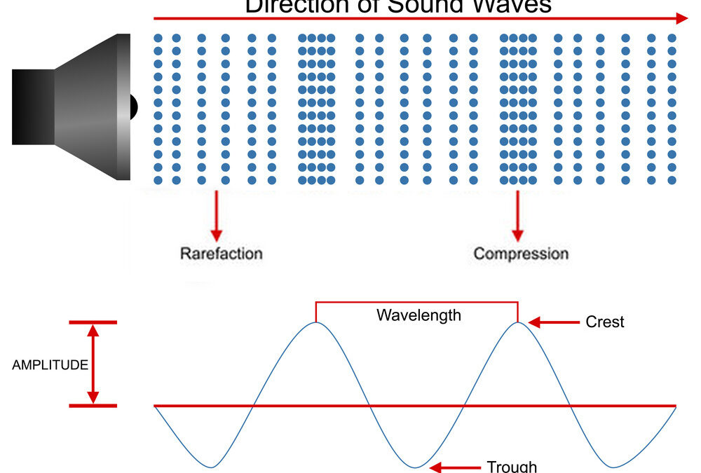
Sound is a good example of a longitudinal wave. The air molecules are pushed back and forth in the same direction that the wave propagates. While sound is normally hard to visualize, we have made an animation to make it easier to see sound in motion. Mouse over the animation below to see the action, mouse off to stop it, and click to restart it.
The animation above shows a rack of squishy balls through which a very slow sound wave is passing. The elephant is causing the wave, which propagates to the right and ends up pushing the man back and forth. The wave causes the balls to move back and forth horizontally, at the same time they are being stretched and compressed. The balls are filled with special gas that changes color when compressed (red) or expanded (blue), making it especially easy for you to follow the action of the waves. This allows you to see the zones of compression and rarefraction (stretching) that are steadily progressing to the right.
We have ignored the process of reflection at the right side and assumed that these waves do not reflect…perhaps because the man is offering just the correct resistance to avoid reflection, so we have a pure traveling (and longitudinal) wave. We will discuss reflections in a later posting. Also, normally sound travels much, much faster than the animation shows. In air it usually travels at about 340 m/s or 1000 ft/s.
If you click on “show graph”, a graph will appear to plot the acoustical pressure in the wave as a function of position. Note that the red pressure maximums line up with the wave crests in the graph. If you click on “show phasors” each ball will have a little phasor vector inside it, indicating the direction of the phasor at that point. (Read other postings on this web site for detailed discussions of phasors.)
On the little phasor diagrams, the real axis is horizontal, pointing to the right, while the imaginary axis is vertical with positive being up. The phasors are indicating the phase of the acoustical pressure wave. Note that the phasors in the red portion of the wave are pointing to the right, at which position the real part is maximum which agrees with the pressure being maximum there.
Likewise, in the blue parts of the wave the phasors are pointing to the left, at which angle the real part of the phasor is most negative corresponding to this negative part of the pressure cycle. Note that we are considering only the changing part of the pressure, call the acoustical pressure, which oscillates positive and negative about the average atmospheric pressure.